Online Bipartite Matching

Introduction

Goal of this is to explain the following paper:

• https://arxiv.org/abs/2005.01929 [Edge-Weighted Online Bipartite Matching], by Matthew Fahrbach, Zhiyi Huang, Runzhou Tao, Morteza Zadimoghaddam

With some more extra reading about variation of OCS (which is being utilized to improve this algorithm)

• https://arxiv.org/abs/2107.02605 [Making Three Out of Two: Three-Way Online Correlated Selection], by Yongho Shin, Hyung-Chan An
• https://ieeexplore.ieee.org/document/9719792/ [Multiway Online Correlated Selection], by Guy Blanc; Moses Charikar

Material

Online Bipartite Matching (Unweighted)

Problem Definition and Score Measurement

• Given a bipartite graph $G = (L \cup R, E)$
• Because it bipartite basically there is no edges between each node in $L$, and each node in $R$.
• Now the matching is I’d say the list of edges being picked, so that each node being incident with at most one edge from the picked edges
• Now the online part is something like the vertex $r$ in the set $R$ is revealed gradually, including the edges incident to $r$
  • L is known in advance, yea
  • Goal is to maximize the cardinality of this matching, which is maximize the side of picked edges.

• There is no rematching, though. However, so if one $r$ is matched, there is no change in the already existing matching.

• it’s said that an algorithm is strictly $\alpha$-competitive if:
  • Expected value of the algorithm that we apply it would be $\ge$ the optimal value for any sequence the order of reveal.

LP Duality

So there’s a video I watch and it mentions about LP Duality, I’m not really strong in this, so might need more inside on linear programming (optimization problem)

LP duality refers to the fact that every linear programming problem has an associated dual problem. The original problem is called the primal problem, and its counterpart is the dual problem.

1. Relationship
   • For every primal problem, there exists a unique dual problem.
2. Structure: If the primal is a maximization problem, the dual is a minimization problem, and vice versa.
3. Weak duality: The objective value of any feasible solution to the dual problem is always a bound on the objective value of the primal problem.
4. Strong duality: Under certain conditions, the optimal objective values of the primal and dual problems are equal.
5. Complementary slackness: This principle helps identify optimal solutions for both primal and dual problems.
6. Economic interpretation: Dual variables often have meaningful economic interpretations, such as shadow prices or opportunity costs.

I’ve seen this problem solved with lagrange multipliers, but already forget some of it, one of the most common solver is z3.

We might seen some of the problem in high school as well, for example when it comes to making cakes, if we make cake type A, it needs F1 flour and C1 egg, if we make type B, we need F2 flour and C2 egg, theres some constraints for example we can only make x amount of cake A, y amount of cake B, or the resources of the flour and egg is limited, thus giving us this optimization problem, something like $F1 + F2 \leq F$ would model the flour and such.

Then we can for example sell this cake for a price, thus giving us the objective.

Greedy Algorithm

Now that we’ve completed our review of LP Duality, let’s discuss the Greedy Algorithm for online bipartite matching:

The greedy algorithm operates as follows:

When an online vertex $r \in R$ arrives:

• If there is an unmatched neighbor in L, match it with the one having the smallest index.

The Greedy Algorithm is strictly $\frac{1}{2}$-competitive.

This competitiveness score implies that for any sequence of vertex arrivals and any possible graph structure that fulfills the requirements (i.e., for any worst-case scenario), the algorithm we apply would achieve at least $\alpha \times opt(G)$, or $OPT \ge ALG \ge \frac{1}{2} \times OPT$ where $opt(G)$ is the maximum matching size for that particular graph G.

We can say that this greedy algorithm is deterministic, so its performance can be relatively easier to compute. For randomized algorithms, however, we approximate $\alpha$ by taking the expected value of the algorithm’s performance. Computing and proving these results for randomized algorithms requires more complex analysis.

To proof this, define the binary cost for each of the node in $L$ and $R$ of our bipartite graph.

$\alpha_l$ = 1 if l is matched in the current matching, 0 otherwise,

For vertices in L:

\[\alpha_l = \begin{cases} 1 & \text{if } l \text{ is matched in the greedy matching} \\ 0 & \text{otherwise} \end{cases}\]

For vertices in R:

\[\beta_r = \begin{cases} 1 & \text{if } r \text{ is matched in the greedy matching} \\ 0 & \text{otherwise} \end{cases}\]

These definitions clearly specify the binary cost for each node in sets L and R of our bipartite graph, based on whether they are matched in the current matching or not. This notation will be useful in proving the competitiveness of the greedy algorithm for online bipartite matching.

It’s true that $\sum_{l\in L}\alpha_l = \sum_{r\in R}\beta_r = ALG$

Claim: $\sum_{l\in L}\alpha_l + \sum_{r\in R}\beta_r \ge $ OPT

Consider any pair $(l, r)$ in $E$, it’s true that $\alpha_l + \beta_r \in {1, 2}$ (otherwise if its unmatched, then just take this edge as part of the matching)

Consider the optimal matching is $OPT \leq \sum_{(l, r) \in OPT}(\alpha_l + \beta_r) \leq \sum_{l \in L}\alpha_l + \sum_{l \in L}\beta_r = 2 \times ALG$

$OPT \leq 2 \times ALG$

$\sum_{(l, r) \in OPT}(\alpha_l + \beta_r)$ one might get confuse by mistaking this as $2\times OPT$, but remember, for $(l, r) \in OPT$, this $(\alpha_l + \beta_r)$ is not necessarily be $2$, because its a greedy match, but we can say for sure at least one of them is matched in their greedy counterparts.

$\square$

Ranking Algorithm

Basically shuffle the $L$ randomly, and apply the greedy algorithm. It will increase the competitive ratio to $1 - \frac{1}{e}$.

If there is 2 complete graph $G = (L, R, E)$, $G^l = (L^l, R, E)$, where $L^l = L \setminus {l}$, for any arbitrary node $l$ in $L$. It’s proven for any step $t$ in the iteration of $R$ addition, define $U^t$ as the set of unmatched node in $L$ during step $t$, and $U^t_l$ as the set of unmatched node in $L^l$ during step $t$, $U^{t}_{l} \sube U^t$.

Proof:

• Imagine $l$ doesn’t have any edge with $r_t$ for the first $n - 1$ steps, $t = {1, 2, 3, \dots, n - 1}$, so WLOG, $U^t = U^t_l \cup {l}$
• Then when the $l$ matches in $G$, it’s either $r_n$ is unmatched in the new graph $G^l$, or it’s matched with another node $l_n$ in $G^l$:

  • if it’s unmatched, then, $U^t = U^t_l$ for the rest of the $t = {n + 1, \dots,

    R

    }$.

  • If it’s matched, then WLOG, we assume $l$ is now that $l_n$, and apply the same proof. (Induction step)

$\square$

Now, generate the indexing as: for each $l \in L$, do a draw $\gamma_l \sim [0, 1]$

Order $L$ by increasing $\gamma_l$. (Basically now its shuffled properly)

if $l$ is matched to $r$: \(\alpha_l = \frac{g(\gamma_l)}{F}\\ \beta_r = \frac{1 - g(\gamma_l)}{F}\) where $g: [0, 1] \rightarrow[0,1], F\in(0, 1]$ are chosen appropriately.

if $l$ is not matched, $\alpha_l = 0$, also if $r$ is not matched, $\beta_r = 0$.

Online Bipartite Matching (Edge Weighted)

Problem Definition and Score Measurement

Basically, now the matching has a score of weight by edge, and want to maximize the sum of edge weights instead.

For easier example models, lets do an input definition on the test cases.

N M E
U[1] V[1] W[1]
U[2] V[2] W[2]
...
U[E] V[E] W[E]

• for $(1 \leq i \leq E)$
  • $1 \leq U[i] \leq N$
  • $1 \leq V[i] \leq M$
  • $0 < W[i]$

2 2 4
1 1 3
2 1 4
2 2 100
1 2 1

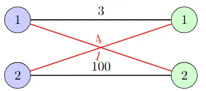
The optimal matching depicted by the black line, while naive greedy would take the pair:

• (2, 1, 4)
• (2, 1, 1)

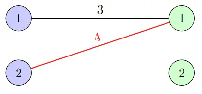
Consider the (1st step) and (2nd step) consecutively revealing $R_1$ and $R_2$

WLOG, let’s assume $R$ is revealed from $1$ to $

R

$.

Now what the free disposal does is, it allows any node in the $l \in L$ to be rematched with the current revealed node at step $t$, $R_t$, disposing $l$’s match if it brings profit for a better match. But it won’t allow the node in the right side to be rematched after disposal

Define an operation $\text{match}_t(x)$ which defines the match decision of node $x$ in the step $t$. e.g: $\text{match}_1(L_2) = R_1$.

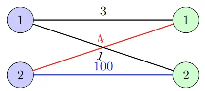
Now free disposal on step-2 allow us two options:

• Dispose $L_2$’s match (2, 1, 4) and take (2, 2, 100) (Bringing +96 profits)
• Take (1, 2, 4) (Bringing +4 profits)

Now it’s intuitive that the greedy decision is just finding the greatest profits among all $l \in L$ that’s connected with $R_t$, to match. Of course, if any matching (including disposal doesn’t bring any profit, then it’s allowed not to match this current $R_t$).

Thus bringing the algorithm to have a reasonable score to measure which brings back us to a similar competitive ratio, the expected value for this current algorithm, over the optimal decision (which can just be done with offline hungarian algorithm).

Submodular Welfare Maximization

We have $n$ agents and $m$ items. Each agent $i$ has a submodular valuation function \(v_i: 2^{[m]} \rightarrow \mathbb{R}_+\) So basically for each agent there is a function that assigns a variation of items that will be valuable. Items arrive online, one at a time. Goal: Allocate items to agents to maximize total value $\sum_{i=1}^n v_i(S_i)$, where $S_i$ is the set of items allocated to agent $i$.

Intuitively, in an offline fashion people would ask several questions:

By logic, the more the items, the more value it would bring (if the $2^{[m]}$ is represented in a DAG, the value would be monotonely non decreasing for each pair of edge, which formally be represented in 2 properties, those are:

1. Submodularity: For any $S \subseteq T$ and element $e$, we have: $v_i(S \cup {e}) - v_i(S) \geq v_i(T \cup {e}) - v_i(T)$

   • Imagine adding toppings to a pizza:

   • The first topping (say, cheese) adds a lot of value.

   • The second topping (maybe pepperoni) adds value, but not as much as the first.

   • Each additional topping adds some value, but less than the previous one.

2. Monotonicity: For any $S \subseteq T$, we have $v_i(S) \leq v_i(T)$

Define:

• $n$: number of agents
• $m$: number of items
• $[m]$: the set of all items, i.e., ${1, 2, …, m}$
• $2^{[m]}$: the power set of $[m]$, i.e., all possible subsets of items
• $v_i: 2^{[m]} \to \mathbb{R}_+$: valuation function for agent $i$
• $S_i$: the set of items allocated to agent $i$

SWM and Bipartite Matching

In bipartite matching:

• $v_i(S) = \max_{j \in S} w_{ij}$
• $w_{ij}$: weight of edge $(i,j)$ in the bipartite graph

Well, if we think about it, Bipartite matching is a special case of SWM where,

• Each agent’s valuation is a unit-demand function
  • $v_i(S) = \max_{j \in S} w_{ij}$, where $w_{ij}$ is the weight of edge $(i,j)$
  • This valuation function is:
    • Submodular: Adding a new item $j$ to $S$ increases the value only if $w_{ij}$ is larger than all previous weights. (Like $+\Delta$)
    • Monotone: Adding an item with a smaller weight doesn’t change the value.

The Greedy Algorithm: A simple greedy algorithm achieves a 1/2-competitive ratio for SWM:

• When item $j$ arrives, allocate it to the agent $i$ that maximizes $v_i(S_i \cup {j}) - v_i(S_i)$

Kapralov, Post, Vondrák proves that this 1/2 ratio is optimal for SWM in the online setting, unless NP = RP.

Key Ideas in the Proof:

1. Reduction from the Max $k$-Cover problem
2. Construction of hard instances that combine:
   • The hardness of approximating Max $k$-Cover
   • The uncertainty in the online setting

Greedy Algorithms

When item $j$ arrives:

• For each agent $i$, compute $\Delta_{ij} = v_i(S_i \cup {j}) - v_i(S_i)$ (This is the marginal value of adding item $j$ to agent $i$’s current set $S_i$)
• Allocate $j$ to agent $i^* = \arg\max_i \Delta_{ij}$

This greedy approach achieves a 1/2-competitive ratio, meaning its solution is always at least half of the optimal offline solution.

Can we do better than this?

Yes, thus we are using the OCS, and to achieve that we can model the problem as a LP problem, and trying to solve it using online primal dual algorithm approach.

References:

• https://www.youtube.com/watch?v=gapQVcEgCMg
• https://arxiv.org/abs/1910.02569
• https://arxiv.org/abs/1910.03287
• https://arxiv.org/abs/1704.05384
• https://www.youtube.com/watch?v=xFZBXshc-FA
• https://arxiv.org/abs/2107.02605

• https://ieeexplore.ieee.org/document/9719792/

• https://i.cs.hku.hk/~zhiyi/file/online-correlated-selection/ocs-cocoon-2024.pdf