Convex Optimizations

Introduction

Convex optimization is a subfield of mathematical optimization that deals with the minimization of convex functions over convex sets.

It’s basically anywhere, even learned while we’re still in high school.

Convex Sets

A set $C$ is convex if, for any two points in the set, the line segment connecting them is also entirely within the set. Mathematically, for any $x_1, x_2 \in C$ and any $\theta$ with $0 \leq \theta \leq 1$, we have:

$\theta x_1 + (1-\theta)x_2 \in C$ (Straight line in any ranked tensor dimension is part of the set as well), $\vec{x}$

Some basic sets:

Lines

Set $C$: The set of all points on a straight line in a 2D plane. Elements: Points $(x, y)$ that satisfy the equation $y = mx + b$, where $m$ is the slope and $b$ is the y-intercept.

Example: $C = {(x, y) \mid y = 2x + 1}$

Here, any two points on this line, say $(0, 1)$ and $(1, 3)$, when connected, will result in a line segment that lies entirely on the line itself. Let’s consider two points on the line $y = 2x + 1$: $x_1 = (0, 1)$ and $x_2 = (1, 3)$

For any $\theta$ between 0 and 1, the point $\theta x_1 + (1-\theta)x_2$ represents a point on the line segment between $x_1$ and $x_2$:

$\theta x_1 + (1-\theta)x_2 = (\theta \cdot 0 + (1-\theta) \cdot 1, \theta \cdot 1 + (1-\theta) \cdot 3)$ $= (1-\theta, 3-2\theta)$

Segments

Set $C$: A portion of a line bounded by two endpoints. Elements: Points $(x, y)$ that lie between and include two specific points.

Example: $C = {(x, y) \mid x = t, y = 2t + 1, \text{ where } 0 \leq t \leq 1}$

This represents a line segment from $(0, 1)$ to $(1, 3)$. Any two points on this segment, when connected, will result in a line segment that is entirely within $C$.

Here, $t$ is actually playing a role similar to $\theta$. Any point on this line segment can be represented as:

$(t, 2t+1) = t(1, 3) + (1-t)(0, 1)$

This is equivalent to $\theta x_2 + (1-\theta)x_1$, where $x_1 = (0, 1)$, $x_2 = (1, 3)$, and $\theta = t$.

The parameter $\theta$ (or $t$ in this case) allows us to describe any point on the line segment as a weighted average of the endpoints. When $\theta = 0$, we get the starting point $(0, 1)$, when $\theta = 1$, we get the ending point $(1, 3)$, and any value in between gives us a point on the line segment.

In essence, $\theta$ acts as a “mixing parameter” that lets us create any point on the line segment by taking a weighted combination of the endpoints. This property is what defines the convexity of the set – any such weighted combination of points in the set must also be in the set.

Circles

Set $C$: All points in a 2D plane at a fixed distance (radius) from a central point. Elements: Points $(x, y)$ that satisfy the equation $(x - h)^2 + (y - k)^2 = r^2$, where $(h, k)$ is the center and $r$ is the radius.

Example: $C = {(x, y) \mid x^2 + y^2 = 1}$

This represents a circle with radius 1 centered at $(0, 0)$. Note that this is actually the boundary of a circle, which is convex. The filled circle (disk) is also convex.

Balls

Set $C$: All points in 3D space within a certain distance (radius) from a central point. Elements: Points $(x, y, z)$ that satisfy the inequality $(x - h)^2 + (y - k)^2 + (z - l)^2 \leq r^2$, where $(h, k, l)$ is the center and $r$ is the radius.

Example: $C = {(x, y, z) \mid x^2 + y^2 + z^2 \leq 1}$

This represents a solid ball with radius 1 centered at $(0, 0, 0)$. Any two points within this ball, when connected, will result in a line segment entirely within the ball.

K Dimensional Linear Object

Set $C$: A XD geometric object with hyperplanes limitations.

Example: $C = {(x, y, z) \mid x \geq 0, y \geq 0, z \geq 0, x + y + z \leq 1}$

This represents a tetrahedron with vertices at $(0, 0, 0)$, $(1, 0, 0)$, $(0, 1, 0)$, and $(0, 0, 1)$. Any two points within or on the surface of this tetrahedron, when connected, will result in a line segment entirely within the tetrahedron.

In each of these examples, you can verify the convexity by taking any two points $x_1$ and $x_2$ in the set $C$ and checking that $\theta x_1 + (1-\theta)x_2$ is also in $C$ for any $\theta$ between 0 and 1. This weighted sum represents any point on the line segment connecting $x_1$ and $x_2$.

Learning about Affine Sets

A set $S$ is affine if for any two points $\mathbf{x}$ and $\mathbf{y}$ in $S$, and any scalar $\theta \in \mathbb{R}$:

$\theta\mathbf{x} + (1-\theta), \mathbf{y} \in S$

^ stolen definition

Function properties:

• Affine functions are both convex and concave
• Convex functions have a unique global minimum (if one exists)

Optimization:

• Affine optimization is a subset of convex optimization
• Convex optimization problems are generally easier to solve than non-convex problems

Dimensionality:

• Affine sets can be thought of as “shifted” linear subspaces
• Convex sets can have curved boundaries

All the other sets:

• Affine Sets
• Convex Sets

Convex Functions

A function $f: \mathbb{R}^n \rightarrow \mathbb{R}$ is convex if its domain is a convex set and for all $x, y$ in the domain of $f$, and $\theta$ with $0 \leq \theta \leq 1$, we have:

$f(\theta x + (1-\theta)y) \leq \theta f(x) + (1-\theta)f(y)$

Geometrically, this means that the line segment between any two points on the graph of the function lies above or on the graph.

Some properties of convex functions:

1. Local minimum is a global minimum
2. The sum of convex functions is convex
3. The maximum of convex functions is convex

There are some extra definitions that are good to take note of:

• $f$ is concave if $-f$ is convex

Some example of the function in $\mathbb{R}^N$ space..

1. Linear functions: Any linear function $f(\mathbf{x}) = \mathbf{a}^T \mathbf{x} + b$, where $\mathbf{a}$ is a vector in $\mathbb{R}^N$ and $b$ is a scalar, is convex.
2. Norm functions:

   • The Euclidean norm $

     \mathbf{x}

     = \sqrt{x_1^2 + x_2^2 + \cdots + x_N^2}$ is convex.

   • Other $p$-norms like the $L_1$ norm (sum of absolute values) are also convex.
3. Quadratic functions: $f(\mathbf{x}) = \mathbf{x}^T A \mathbf{x} + \mathbf{b}^T \mathbf{x} + c$, where $A$ is a positive semidefinite matrix, $\mathbf{b}$ is a vector, and $c$ is a scalar.
4. Exponential function: $f(\mathbf{x}) = e^{\mathbf{a}^T \mathbf{x}}$, where $\mathbf{a}$ is a vector in $\mathbb{R}^N$.
5. Log-sum-exp function: $f(\mathbf{x}) = \log(e^{x_1} + e^{x_2} + \cdots + e^{x_N})$
6. Maximum function: $f(\mathbf{x}) = \max{x_1, x_2, \ldots, x_N}$
7. Distance to a convex set: If $C$ is a convex set in $\mathbb{R}^N$, then $f(\mathbf{x}) = \min{|\mathbf{x} - \mathbf{y}| : \mathbf{y} \in C}$ is convex.
8. Composition with affine mapping: If $g: \mathbb{R}^M \to \mathbb{R}$ is convex and $A$ is an $N \times M$ matrix, then $f(\mathbf{x}) = g(A\mathbf{x})$ is convex on $\mathbb{R}^N$.

Extended-Value Extension (TL:DR extending domain)

Basic Concept

The extended-value extension is a way to extend a function defined on a subset of $\mathbb{R}^n$ to the entire space $\mathbb{R}^n$ by assigning the value $+\infty$ to points outside the original domain.

Formal Definition

Given a function $f: D \to \mathbb{R}$, where $D \subseteq \mathbb{R}^n$, the extended-value extension $\bar{f}: \mathbb{R}^n \to \mathbb{R} \cup {+\infty}$ is defined as: \(\bar{f}(x) =\begin{cases} f(x) & \text{if } x \in D \\ +\infty & \text{if } x \notin D \end{cases}\)

Importance-and Applications

1. Domain Representation: It allows us to implicitly represent the domain of a function within the function itself.
2. Convexity Preservation: If $f$ is convex on $D$, then $\bar{f}$ is convex on $\mathbb{R}^n$.
3. Optimization: It’s particularly useful in optimization problems, allowing us to incorporate constraints into the objective function.
4. Simplification: It often simplifies the statement and analysis of optimization problems.
5. Duality Theory: It plays a crucial role in duality theory and the formulation of Lagrangian dual problems.

Example

Consider the function $f(x) = \log x$ defined on $(0,\infty)$. Its extended-value extension is: \(\bar{f}(x) = \begin{cases} \log x & \text{if } x > 0 \\ +\infty & \text{if } x \leq 0 \end{cases}\)

This extension preserves the convexity of the original logarithm function while extending its domain to all of $\mathbb{R}$.

Properties

1. Lower Semicontinuity: The extended-value extension of a continuous function is always lower semicontinuous.
2. Epigraph: The epigraph of $\bar{f}$ is the closure of the epigraph of $f$. (will talk in the next section)
3. Indicator Functions: The indicator function of a set is a special case of an extended-value extension.

The extended-value extension is a powerful tool in convex analysis, allowing us to work with functions on the entire space $\mathbb{R}^n$ while preserving important properties like convexity. It’s particularly useful in optimization theory, where it allows us to elegantly handle constraints and develop duality results.

First-Order Condition for Convexity

The first-order condition relates to the gradient of a differentiable function.

Definition

For a differentiable function $f: \mathbb{R}^n \to \mathbb{R}$, $f$ is convex if and only if for all $x, y \in \text{dom}(f)$:

$f(y) \geq f(x) + \nabla f(x)^T(y-x)$

$\nabla f(x)$

• This is the gradient of $f$ at point $x$.
• For a function $f: \mathbb{R}^n \to \mathbb{R}$, the gradient is an n-dimensional vector of partial derivatives: $\nabla f(x) = (\frac{\partial f}{\partial x_1}, \frac{\partial f}{\partial x_2}, …, \frac{\partial f}{\partial x_n})$

This condition states that the first-order Taylor approximation of $f$ at any point $x$ is a global underestimator of $f$.

Second-Order Condition for Convexity

The second-order condition involves the Hessian matrix of a twice-differentiable function.

Definition

For a twice-differentiable function $f: \mathbb{R}^n \to \mathbb{R}$, $f$ is convex if and only if its Hessian matrix $\nabla^2 f(x)$ is positive semidefinite for all $x \in \text{dom}(f)$.

This means that for all $x$ and $v$:

$v^T \nabla^2 f(x) v \geq 0$

Talking about Hessian and Jacobian

Jacobian Matrix

The Jacobian is a generalization of the gradient for vector-valued functions.

Definition

For a function $\mathbf{f}: \mathbb{R}^n \to \mathbb{R}^m$ with components $(f_1, …, f_m)$, the Jacobian matrix $J$ is an $m \times n$ matrix of all first-order partial derivatives: \(J = \begin{bmatrix} \frac{\partial f_1}{\partial x_1} & \cdots & \frac{\partial f_1}{\partial x_n} \\ \vdots & \ddots & \vdots \\ \frac{\partial f_m}{\partial x_1} & \cdots & \frac{\partial f_m}{\partial x_n} \end{bmatrix}\)

Properties

1. If $m = 1$ (i.e., $f$ is scalar-valued), the Jacobian is equivalent to the gradient, transposed.
2. The Jacobian represents the best linear approximation to a differentiable function near a given point.

Applications

1. Used in the multivariable chain rule
2. Important in the study of vector fields
3. Used in transformations between coordinate systems

Hessian Matrix

The Hessian is a square matrix of second-order partial derivatives of a scalar-valued function.

Definition

For a function $f: \mathbb{R}^n \to \mathbb{R}$, the Hessian matrix $H$ is an $n \times n$ symmetric matrix:

\[H = \begin{bmatrix} \frac{\partial^2 f}{\partial x_1^2} & \frac{\partial^2 f}{\partial x_1 \partial x_2} & \cdots & \frac{\partial^2 f}{\partial x_1 \partial x_n} \\ \frac{\partial^2 f}{\partial x_2 \partial x_1} & \frac{\partial^2 f}{\partial x_2^2} & \cdots & \frac{\partial^2 f}{\partial x_2 \partial x_n} \\ \vdots & \vdots & \ddots & \vdots \\ \frac{\partial^2 f}{\partial x_n \partial x_1} & \frac{\partial^2 f}{\partial x_n \partial x_2} & \cdots & \frac{\partial^2 f}{\partial x_n^2} \end{bmatrix}\]

Properties

1. The Hessian is symmetric if the function is twice continuously differentiable (due to Clairaut’s theorem).
2. The determinant of the Hessian is used in the second derivative test for determining critical points.
3. For a twice differentiable function, convexity can be characterized by the positive semidefiniteness of its Hessian.

Applications

1. Used in optimization to determine the nature of critical points (minima, maxima, or saddle points).
2. Important in the study of curvature of surfaces.
3. Used in the second-order Taylor approximation of functions.

Relationship between Jacobian and Hessian

1. The Hessian of a scalar-valued function is the Jacobian of its gradient.
2. For a vector-valued function $\mathbf{f}: \mathbb{R}^n \to \mathbb{R}^m$, we can consider the Hessian of each component function $f_i$. This gives us $m$ different Hessian matrices, each of size $n \times n$.

Both the Jacobian and Hessian play crucial roles in optimization algorithms, particularly in methods like Newton’s method for finding roots or minima of functions. They provide important information about the local behavior of functions, which is essential for many numerical methods and theoretical analyses in applied mathematics and related fields.

Epigraph

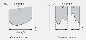
The epigraph of a function $f: \mathbb{R}^n \to \mathbb{R}$ is the set of points lying on or above its graph:

$\text{epi}(f) = {(x,t) \in \mathbb{R}^{n+1} : x \in \text{dom}(f), t \geq f(x)}$

A function is convex if and only if its epigraph is a convex set.

Sublevel Set

The $\alpha$-sublevel set of a function $f: \mathbb{R}^n \to \mathbb{R}$ is:

$S_\alpha = {x \in \text{dom}(f) : f(x) \leq \alpha}$

Property

If $f$ is convex, then all its sublevel sets are convex.

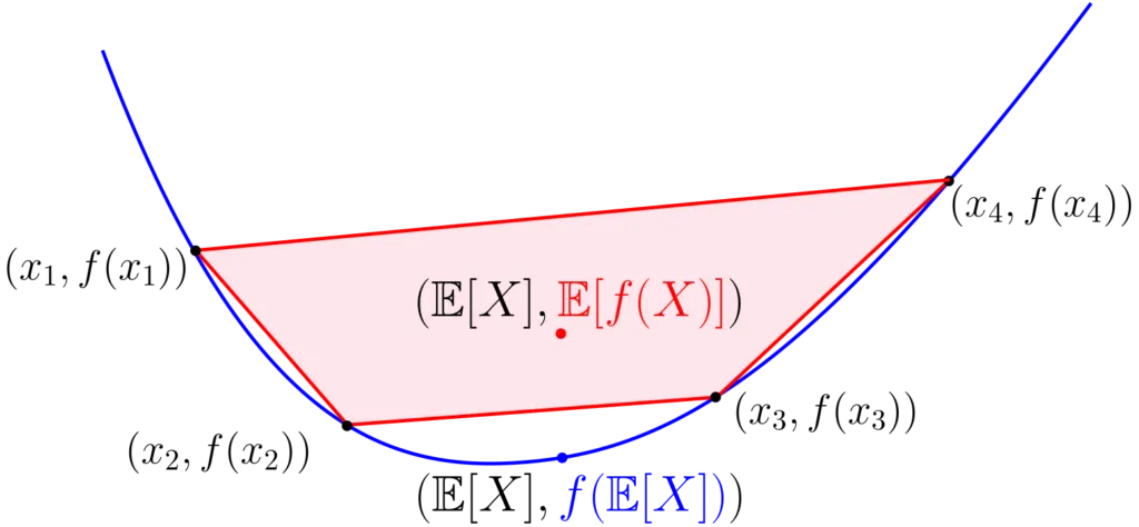
Jensen’s Inequality

Jensen’s inequality is a fundamental property of convex functions.

Definition

For a convex function $f$ and points $x_1, \ldots, x_n$ in its domain, and non-negative weights $\lambda_1, \ldots, \lambda_n$ that sum to 1:

$f(\sum_{i=1}^n \lambda_i x_i) \leq \sum_{i=1}^n \lambda_i f(x_i)$

Interpretation

The function value at the weighted average of points is less than or equal to the weighted average of function values at those points.

Imagine you have a convex function (think of a U-shaped curve) and you pick some points on this curve.

1. If you average these points and then apply the function to this average, you get one result.
2. If you apply the function to each point separately and then average these results, you get another result.

Jensen’s inequality states that the first result (function of the average) will always be less than or equal to the second result (average of the functions).

Think of a hammock hanging between two trees:

• The trees represent two points on your convex function.
• The straight line of the hammock represents the average between these points.
• The curve of the function will always be above or touching this straight line, never below it.

Let’s use $f(x) = x^2$ as our convex function:

1. Take two numbers: 1 and 3, 2
2. $f(2) = 2^2 = 4$ (function of the average)
3. $f(1) = 1^2 = 1$ and $f(3) = 3^2 = 9$
4. Average of these: (1 + 9) / 2 = 5 (average of the functions)

Jensen’s inequality says: $f(\text{average}) \leq \text{average}(f)$ In this case: 4 ≤ 5, which is true!

Here is a better illustration, stolen from https://francisbach.com/jensen-inequality/

Special Case

For $n=2$ and $\lambda_1 = \lambda_2 = \frac{1}{2}$, we get:

$f(\frac{x+y}{2}) \leq \frac{f(x) + f(y)}{2}$

This illustrates that the midpoint of a chord lies above or on the graph of a convex function.

These concepts are interconnected and fundamental to understanding convex functions and their properties. They play crucial roles in optimization theory, machine learning, and many other fields where convex analysis is applied.

I’m gonna skip some crazy explanation here, but let’s just get to duality problem, which is a framework to solve optimization problems

Duality Problem

Duality is a damn strong concept in optimization that provides an alternative perspective on optimization problems.

It allows us to transform a primal problem (usually a minimization problem) into a dual problem (usually a maximization problem).

.. It doesn’t have anything to do with yin and yang

This transformation can often lead to simpler solutions or provide additional insights into the problem structure.

Key Components:

1. Primal Problem: The original optimization problem we want to solve.
2. Lagrangian Function: A function that combines the objective and constraints.
3. Dual Function: Derived from the Lagrangian, it provides a lower bound on the primal objective.
4. Dual Problem: An optimization problem based on the dual function.

By the way, all variables we’re talking about here is a vector.

Let’s break this down step by step:

Primal Problem

The general form of a primal problem is:

• minimize $f_0(x)$
• subject to $f_i(x) \leq 0$, for $i = 1, …, m$
• $h_j(x) = 0$, for $j = 1, …, p$

Why is it called primal? Because this is equations that were given when you trying to solve optimization problems.

Here, $x$ is the optimization variable, $f_0(x)$ is the objective function, $f_i(x)$ are inequality constraints, and $h_j(x)$ are equality constraints.

Lagrangian Function

The Lagrangian combines the objective function and constraints:

$L(x, \lambda, \nu) = f_0(x) + \sum_{i=1}^m \lambda_i f_i(x) + \sum_{j=1}^p \nu_j h_j(x)$

Where $\lambda_i \geq 0$ are called Lagrange multipliers for inequality constraints, and $\nu_j$ are Lagrange multipliers for equality constraints.

Alright, so this is why you dont go to Cinema when you have Calculus 2 class.

What is it?

The Lagrangian is a way to solve optimization problems with constraints. It’s like solving a puzzle where you want to find the best solution while following certain rules.

Imagine you’re on a hill (your function) and you’re trying to find the highest point, but you’re restricted to stay on a specific path (your constraint).

1. Function: Let’s call the function you want to optimize $f(x,y)$. This is your “hill”.
2. Constraint: The restriction is another function, say $g(x,y) = c$. This is your “path”.
3. The Key Insight: At the point where $f$ reaches its maximum or minimum along the constraint, the gradients of $f$ and $g$ are parallel.

The core idea is expressed mathematically as:

$\nabla f = \lambda \nabla g$

Where:

• $\nabla f$ is the gradient of your function
• $\nabla g$ is the gradient of your constraint
• $\lambda$ is the Lagrange multiplier

The $\lambda$ (Lagrange multiplier) tells you how much the optimal value of $f$ would change if you relaxed the constraint a little bit.

It’s like finding where the contour lines of $f$ just touch the constraint curve.

1. Write out the equation $\nabla f = \lambda \nabla g$
2. Use this along with your constraint equation $g(x,y) = c$
3. Solve these equations together to find the optimal points

Lmao: https://tutorial.math.lamar.edu/Classes/CalcIII/LagrangeMultipliers.aspx

Think about lagrangian is basically solving the equation for the ones that stays in the boundary of the equality (actually if there is a gap in the solution, e.g an equation)

The Parts:

1. $f_0(x)$ - This is what you’re trying to optimize (minimize or maximize). Think of it as your main goal.
2. $\sum_{i=1}^m \lambda_i f_i(x)$ - These are the inequality constraints. Think of them as “less than or equal to” rules.
3. $\sum_{j=1}^p \nu_j h_j(x)$ - These are the equality constraints. Think of them as “must be equal to” rules.
4. $\lambda_i$ and $\nu_j$ - These are called Lagrange multipliers. Think of them as weights that balance the importance of each constraint.

Dual Function

The dual function is defined as the infimum (greatest lower bound) of the Lagrangian over x:

$g(\lambda, \nu) = \inf_x L(x, \lambda, \nu)$

Where:

• $L(x, \lambda, \nu)$ is the Lagrangian function
• $\inf_x$ denotes the infimum (greatest lower bound) with respect to $x$

Infimum Operation:

• We’re finding the smallest value of $L$ over all possible $x$, for fixed $\lambda$ and $\nu$.
• This operation “eliminates” the primal variable $x$.

Domain:

• $g(\lambda, \nu)$ is defined for all $\lambda \in \mathbb{R}^m$ and $\nu \in \mathbb{R}^p$.
• However, it’s only meaningful when $\lambda \geq 0$ for inequality constraints.

Concavity:

• $g(\lambda, \nu)$ is always concave, even if the original problem is not convex.
• This is because it’s the pointwise infimum of affine functions of $(\lambda, \nu)$.

Lower Bound Property:

• For any feasible $x$ and any $\lambda \geq 0$, $\nu$: $g(\lambda, \nu) \leq f_0(x)$

If we get back to the basic, see this problem:

Minimize $f(x,y)$ subject to $g(x,y) = c$

The Lagrangian for this problem is:

$L(x, y, \lambda) = f(x,y) + \lambda(g(x,y) - c)$

Where:

• $f(x,y)$ is the objective function
• $g(x,y) = c$ is the constraint
• $\lambda$ is the Lagrange multiplier

See how:

1. Unconstrained Optimization: The Lagrangian turns a constrained problem into an unconstrained one.

2. Penalty Interpretation:

   • $\lambda(g(x,y) - c)$ acts as a penalty term.
   • When the constraint is satisfied, this term is zero.
   • When the constraint is violated, this term is non-zero.

3. Finding Critical Points: We find critical points by setting partial derivatives to zero:

   $\frac{\partial L}{\partial x} = 0$, $\frac{\partial L}{\partial y} = 0$, $\frac{\partial L}{\partial \lambda} = 0$

4. Geometric Interpretation: At the optimum, the gradients of $f$ and $g$ are parallel:

   $\nabla f = -\lambda \nabla g$

The dual function $g(\lambda)$ is the infimum of $L$ with respect to $x$ and $y$:

$g(\lambda) = \inf_{x,y} L(x, y, \lambda)$

Dual Problem

The dual problem is then formulated as:

maximize $g(\lambda, \nu)$, subject to $\lambda \geq 0$

What does the above mean (Recap), intro to Duality gap and KKT Condition

The dual function is defined as:

$g(\lambda, \nu) = \inf_x L(x, \lambda, \nu)$

• This operation finds the smallest value of the Lagrangian for any given $\lambda$ and $\nu$.
• It’s like finding the “worst-case scenario” (lowest value) for each set of multipliers.
• This process effectively eliminates the primal variables $(x)$, transforming the problem into one over $\lambda$ and $\nu$.
• In basic calculus, we often dealt only with equality constraints using Lagrange multipliers.
• The dual function generalizes this to include inequality constraints (associated with $\lambda \geq 0$).
• The principle remains similar: we’re finding points where the objective function is tangent to the constraint surfaces, but now in a more general setting.

$g(\lambda, \nu) \leq f_0(x^)$ for any feasible $x^$

• This is crucial: the dual function always provides a lower bound on the optimal primal value.
• It’s true because: a) For feasible $x^$, all constraints are satisfied, so $L(x^, \lambda, \nu) = f_0(x^)$ for $\lambda \geq 0$. b) The infimum over all $x$ must be less than or equal to the value at any specific $x^$.

maximize $g(\lambda, \nu)$, subject to $\lambda \geq 0$

• We’re seeking the best (highest) lower bound on the primal optimal value.
• This turns the original minimization problem into a maximization problem.
• The constraint $\lambda \geq 0$ ensures we’re only considering valid lower bounds.

Duality Gap: The difference between the primal optimal value and the dual optimal value is called the duality gap. When this gap is zero (strong duality), solving the dual problem effectively solves the primal problem.

Computational Advantage: Often, the dual problem is easier to solve than the primal problem, especially when there are fewer dual variables than primal variables.

Sensitivity Analysis: The optimal dual variables ($\lambda^, \nu^$) provide information about how the optimal value changes with respect to the constraints.

Convexity: The dual function is always concave, even if the original problem is not convex. This can make the dual problem easier to solve.

Feasibility: Any dual feasible solution provides a lower bound on the primal optimal value, which can be useful even if we can’t solve the primal problem exactly.

KKT Conditions: The relationship between primal and dual problems leads to the Karush-Kuhn-Tucker (KKT) conditions, which are necessary (and often sufficient) conditions for optimality in nonlinear programming.

$\max_{\lambda \geq 0, \nu} \inf_x L(x, \lambda, \nu) \leq \min_x \sup_{\lambda \geq 0, \nu} L(x, \lambda, \nu)$

• Left side: Dual problem (maximization)
• Right side: Primal problem (minimization)
• This inequality is known as weak duality

Duality Gap

A duality gap occurs when the optimal value of the dual problem is not equal to the optimal value of the primal problem.

• Strong duality: $p^* = d^*$
• Weak duality: $d^* \leq p^*$ (for minimization problems)

Where $p^\star$ is the optimal value of the primal problem and $d^\star$ is the optimal value of the dual problem.

When There’s a Gap

• A gap usually indicates that the problem is not convex or that some constraint qualifications are not met.

• In such cases, solving the dual problem may not give you the exact solution to the primal problem.

• However, it can still provide a bound on the optimal value:

  $d^* \leq p^*$

Practical Implications

• With strong duality $(p^* = d^*)$, you can often solve the dual problem instead of the primal, which is sometimes easier.
• Even with a gap, the dual problem can provide useful bounds and insights.

More on Duality

https://www.youtube.com/watch?v=ZGjBeX0iY2w

Examples

Primal Problem: Minimize $f(x) = x^2 + 1$ Subject to: $x \geq 2$

1. Form the Lagrangian: $L(x, \lambda) = x^2 + 1 + \lambda(2 - x)$

2. To find the infimum for the dual function: $g(\lambda) = \inf_x L(x, \lambda)$

   We use the gradient (first derivative) with respect to x:

   $\frac{\partial L}{\partial x} = 2x - \lambda = 0$

3. Solve this equation: $2x - \lambda = 0$ $x = \frac{\lambda}{2}$

4. This gives us the x that minimizes L for any given λ. We then substitute this back into L to get g(λ):

   $g(\lambda) = (\frac{\lambda}{2})^2 + 1 + \lambda(2 - \frac{\lambda}{2})$ $= \frac{\lambda^2}{4} + 1 + 2\lambda - \frac{\lambda^2}{2}$ $= -\frac{\lambda^2}{4} + 2\lambda + 1$

I apologize for the misunderstanding. You’re right, let’s present this using LaTeX-flavored Markdown. This format is indeed more suitable for many online platforms and documentation systems.

Weak Duality: $d^* \leq p^*$

\[\begin{aligned} \text{Minimize } & z = 2x + 3y \\ \text{Subject to: } & x + y \geq 4 \\ & x, y \geq 0 \end{aligned}\]

Step 1: Lagrangian

\(L(x, y, \lambda) = 2x + 3y + \lambda(4 - x - y)\)

Step 2: Dual Function

\(\begin{aligned} g(\lambda) &= \inf\{L(x, y, \lambda) : x, y \geq 0\} \\ &= \inf\{(2-\lambda)x + (3-\lambda)y + 4\lambda : x, y \geq 0\} \end{aligned}\)

Step 3: Analyze $g(\lambda)$

\(g(\lambda) = \begin{cases} 4\lambda & \text{if } \lambda \leq 2 \text{ and } \lambda \leq 3 \\ -\infty & \text{otherwise} \end{cases}\)

Step 4: Dual Problem

\(\begin{aligned} \text{Maximize } & 4\lambda \\ \text{Subject to: } & \lambda \leq 2 \\ & \lambda \leq 3 \\ & \lambda \geq 0 \end{aligned}\)

Step 5: Solutions

Primal solution: $x = 4, y = 0, p^* = 8$ Dual solution: $\lambda = 2, d^* = 8$

Strong duality holds: $d^* = p^* = 8$

Weak Duality Example

Modified Primal Problem

\(\begin{aligned} \text{Minimize } & z = 2x + 3y \\ \text{Subject to: } & x + y \geq 4 \\ & x, y \geq 0 \\ & x, y \text{ are integers} \end{aligned}\)

Dual Problem (unchanged)

\(\begin{aligned} \text{Maximize } & 4\lambda \\ \text{Subject to: } & \lambda \leq 2 \\ & \lambda \leq 3 \\ & \lambda \geq 0 \end{aligned}\)

Solutions

Primal solution:

\[p^* = \infty\]

Dual solution: \(\lambda = 2\) \(d^* = 4(2) = 8\)

Weak duality holds: $d^* \leq p^*$

Key Points

1. Weak Duality: $d^* \leq p^*$
   • Always holds
   • The dual provides a lower bound on the primal optimal value
2. Strong Duality: $d^* = p^*$
   • Holds under certain conditions (e.g., Slater’s condition for convex problems)
   • Provides exact solution and sensitivity information
3. Duality Gap: $p^* - d^*$
   • In weak duality: $p^* - d^* > 0$
   • In strong duality: $p^* - d^* = 0$
4. Importance of Weak Duality:
   • Even when $d^* < p^*$, the dual problem provides a useful bound
   • In algorithm design: $d^* \leq \text{optimal} \leq \text{current feasible solution}$

More on Karush-Kuhn-Tucker (KKT) Conditions

The KKT conditions are first-order necessary conditions for a solution in nonlinear programming to be optimal. They generalize the method of Lagrange multipliers to inequality constraints.

General Problem Formulation

Consider the optimization problem:

\[\begin{aligned} \text{Minimize } & f(x) \\ \text{Subject to: } & g_i(x) \leq 0, \quad i = 1, \ldots, m \\ & h_j(x) = 0, \quad j = 1, \ldots, p \end{aligned}\]

Where $x \in \mathbb{R}^n$, $f$ is the objective function, $g_i$ are inequality constraints, and $h_j$ are equality constraints.

KKT Conditions

For a solution $x^*$ to be optimal, it must satisfy the following conditions:

1. Stationarity: \(\nabla f(x^*) + \sum_{i=1}^m \lambda_i \nabla g_i(x^*) + \sum_{j=1}^p \mu_j \nabla h_j(x^*) = 0\)

2. Primal Feasibility: \(g_i(x^*) \leq 0, \quad i = 1, \ldots, m\) \(h_j(x^*) = 0, \quad j = 1, \ldots, p\)

3. Dual Feasibility: \(\lambda_i \geq 0, \quad i = 1, \ldots, m\)

4. Complementary Slackness: \(\lambda_i g_i(x^*) = 0, \quad i = 1, \ldots, m\)

Here, $\lambda_i$ and $\mu_j$ are the KKT multipliers (or Lagrange multipliers).

Interpretation of KKT Conditions

1. Stationarity: At the optimal point, the gradients of the objective and active constraints are linearly dependent.

2. Primal Feasibility: The solution must satisfy all constraints.

3. Dual Feasibility: The multipliers for inequality constraints must be non-negative.

4. Complementary Slackness: For each inequality constraint, either the constraint is active ($g_i(x^*) = 0$) or its multiplier is zero ($\lambda_i = 0$).

Importance of KKT Conditions

1. Optimality Criteria: They provide necessary conditions for optimality in nonlinear programming.

2. Duality Connection: KKT conditions bridge primal and dual problems, relating to strong duality.

3. Algorithm Design: Many optimization algorithms are designed to find points satisfying KKT conditions.

4. Economic Interpretation: In economics, KKT multipliers often represent shadow prices or marginal values.

Limitations

• KKT conditions are necessary but not always sufficient for optimality.
• They assume certain regularity conditions (constraint qualifications) are met.

Example Application

Consider a simple problem:

\[\begin{aligned} \text{Minimize } & f(x, y) = x^2 + y^2 \\ \text{Subject to: } & x + y - 1 \geq 0 \end{aligned}\]

Applying KKT:

1. Stationarity: $2x + \lambda = 0$, $2y + \lambda = 0$
2. Primal Feasibility: $x + y - 1 \geq 0$
3. Dual Feasibility: $\lambda \geq 0$
4. Complementary Slackness: $\lambda(x + y - 1) = 0$

Solving these equations leads to the optimal solution: $x^* = y^* = \frac{1}{2}$, $\lambda^* = 1$.